
Mastering Custom SageMaker Deployment: A Comprehensive Guide
A deep dive into the intricacies of deploying custom models to Amazon SageMaker

This notebook classifies credit card transactions to fraudulent or non fraudulent, the dataset is a set of PCA features extracted from the original data in order to conceal the identities of the parties in question.
# install torchsummary
!pip install -q torchsummary
[33mWARNING: Running pip as root will break packages and permissions. You should install packages reliably by using venv: https://pip.pypa.io/warnings/venv[0m
import torch
import torch.nn as nn
import pandas as pd
import matplotlib.pyplot as plt
import seaborn as sns
from numpy import sum
from sklearn.metrics import confusion_matrix, classification_report
from sklearn.model_selection import train_test_split
from sklearn.preprocessing import StandardScaler
from torch.utils.data import TensorDataset, DataLoader
from tqdm import tqdm
from torchsummary import summary

# set figure size
plt.rcParams["figure.figsize"] = (14,7)
df = pd.read_csv("../input/creditcardfraud/creditcard.csv")
df.head()
| Time | V1 | V2 | V3 | V4 | V5 | V6 | V7 | V8 | V9 | ... | V21 | V22 | V23 | V24 | V25 | V26 | V27 | V28 | Amount | Class | |
|---|---|---|---|---|---|---|---|---|---|---|---|---|---|---|---|---|---|---|---|---|---|
| 0 | 0.0 | -1.359807 | -0.072781 | 2.536347 | 1.378155 | -0.338321 | 0.462388 | 0.239599 | 0.098698 | 0.363787 | ... | -0.018307 | 0.277838 | -0.110474 | 0.066928 | 0.128539 | -0.189115 | 0.133558 | -0.021053 | 149.62 | 0 |
| 1 | 0.0 | 1.191857 | 0.266151 | 0.166480 | 0.448154 | 0.060018 | -0.082361 | -0.078803 | 0.085102 | -0.255425 | ... | -0.225775 | -0.638672 | 0.101288 | -0.339846 | 0.167170 | 0.125895 | -0.008983 | 0.014724 | 2.69 | 0 |
| 2 | 1.0 | -1.358354 | -1.340163 | 1.773209 | 0.379780 | -0.503198 | 1.800499 | 0.791461 | 0.247676 | -1.514654 | ... | 0.247998 | 0.771679 | 0.909412 | -0.689281 | -0.327642 | -0.139097 | -0.055353 | -0.059752 | 378.66 | 0 |
| 3 | 1.0 | -0.966272 | -0.185226 | 1.792993 | -0.863291 | -0.010309 | 1.247203 | 0.237609 | 0.377436 | -1.387024 | ... | -0.108300 | 0.005274 | -0.190321 | -1.175575 | 0.647376 | -0.221929 | 0.062723 | 0.061458 | 123.50 | 0 |
| 4 | 2.0 | -1.158233 | 0.877737 | 1.548718 | 0.403034 | -0.407193 | 0.095921 | 0.592941 | -0.270533 | 0.817739 | ... | -0.009431 | 0.798278 | -0.137458 | 0.141267 | -0.206010 | 0.502292 | 0.219422 | 0.215153 | 69.99 | 0 |
5 rows × 31 columns
# some stats about the data
print(f"Number of data points: {df.size}")
print(f"Number of Fradulant Transactions: {df['Class'].value_counts()[1]}")
print(f"Number of non-fradulant Transactions: {df['Class'].value_counts()[0]}\n\n")
sns.countplot(x=df["Class"], palette="YlGnBu").set(title="Class Balance Between Transcation Types")
plt.show()
Number of data points: 8829017
Number of Fradulant Transactions: 492
Number of non-fradulant Transactions: 284315
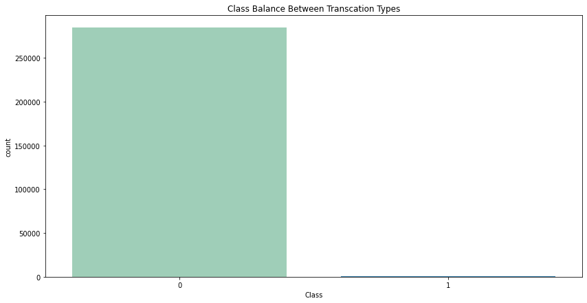
there is huge class impalance in the data, this might lead to a biased model, we can mitigate this by only using the same amount of class 0 while training or we could generate some sample data from the given features.
# Amount per transaction for each type
sns.scatterplot(data=df.reset_index(), x="index", y="Amount", hue="Class", cmap="YlGnBu").set(title="Amount per transaction")
plt.show()
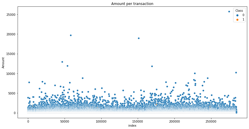
fraudulent transactions dont tend to have a large sum of cash per transaction, we can confirm this by calculating some statistics such as max, min and mean for each type of transaction.
for i, word in zip(range(2), ["Positive", "Negative"]):
    print(f"{word} transactions statistics")
    print(df[df["Class"] == i]["Amount"].describe(), "\n\n")
Positive transactions statistics
count    284315.000000
mean         88.291022
std         250.105092
min           0.000000
25%           5.650000
50%          22.000000
75%          77.050000
max       25691.160000
Name: Amount, dtype: float64


Negative transactions statistics
count     492.000000
mean      122.211321
std       256.683288
min         0.000000
25%         1.000000
50%         9.250000
75%       105.890000
max      2125.870000
Name: Amount, dtype: float64
# split data into training and testing
X = df.drop("Class", axis=1)
y = df["Class"]

# scale the values of x (better training)
scaler = StandardScaler()
scaler.fit(X)
X = scaler.transform(X)

# split data to train and test
X_train, X_test, y_train, y_test = train_test_split(X, y, test_size=0.30, stratify=y) # stratify keeps class balance
# create tensor datasets from df
X_train = torch.FloatTensor(X_train)
X_test = torch.FloatTensor(X_test)
y_train = torch.FloatTensor(y_train.values)
y_test = torch.FloatTensor(y_test.values)
train_ds = TensorDataset(X_train, y_train)
device = 'cuda' if torch.cuda.is_available() else 'cpu'
print(device)
cuda
# create dataloaders
batch_size = 128
train_dl = DataLoader(train_ds, batch_size=batch_size)
# Network Architecture
class FraudNet(nn.Module):
    def __init__(self, input_dim, hidden_dim, num_layers=4):
        super().__init__()
        self.input = nn.Sequential(
            nn.Linear(input_dim, hidden_dim),
            nn.ReLU()
        )
        # make the number of hidden dim layers configurable
        self.layers = nn.ModuleList()
        for i in range(num_layers):
            self.layers.append(nn.Linear(hidden_dim, hidden_dim))
            self.layers.append(nn.ReLU())

        # final layer
        self.fc = nn.Linear(hidden_dim, 2)

    def forward(self, x):
        out = self.input(x)
        for layer in self.layers:
            out = layer(out)
        return self.fc(out)
# training function
def train_model(model, epochs, loss_fn, optimizer):
    model.train()
    for epoch in range(epochs):
        with tqdm(train_dl, unit="batch") as tepoch:
            for data, target in tepoch:
                data, target = data.to(device), target.to(device)
                tepoch.set_description(f"Epoch {epoch}")
                optimizer.zero_grad()
                preds = model(data)
                loss = loss_fn(preds, target.long())
                loss.backward()
                optimizer.step()
                tepoch.set_postfix(loss=loss.item())
inp_size = X_train.shape[1]
model = FraudNet(inp_size, inp_size).to(device)
loss = nn.CrossEntropyLoss()
optim = torch.optim.Adam(model.parameters(),  lr = 1e-4)

# summarize the model layers
summary(model, (inp_size, inp_size))
----------------------------------------------------------------
        Layer (type)               Output Shape         Param #
================================================================
            Linear-1               [-1, 30, 30]             930
              ReLU-2               [-1, 30, 30]               0
            Linear-3               [-1, 30, 30]             930
              ReLU-4               [-1, 30, 30]               0
            Linear-5               [-1, 30, 30]             930
              ReLU-6               [-1, 30, 30]               0
            Linear-7               [-1, 30, 30]             930
              ReLU-8               [-1, 30, 30]               0
            Linear-9               [-1, 30, 30]             930
             ReLU-10               [-1, 30, 30]               0
           Linear-11                [-1, 30, 2]              62
================================================================
Total params: 4,712
Trainable params: 4,712
Non-trainable params: 0
----------------------------------------------------------------
Input size (MB): 0.00
Forward/backward pass size (MB): 0.07
Params size (MB): 0.02
Estimated Total Size (MB): 0.09
----------------------------------------------------------------
epochs = 10
train_model(model, epochs, loss, optim)
Epoch 0: 100%|██████████| 1558/1558 [00:11<00:00, 137.25batch/s, loss=0.000822]
Epoch 1: 100%|██████████| 1558/1558 [00:11<00:00, 138.96batch/s, loss=0.000756]
Epoch 2: 100%|██████████| 1558/1558 [00:11<00:00, 139.36batch/s, loss=0.0022]
Epoch 3: 100%|██████████| 1558/1558 [00:11<00:00, 133.62batch/s, loss=0.00293]
Epoch 4: 100%|██████████| 1558/1558 [00:11<00:00, 137.87batch/s, loss=0.00276]
Epoch 5: 100%|██████████| 1558/1558 [00:11<00:00, 137.02batch/s, loss=0.00241]
Epoch 6: 100%|██████████| 1558/1558 [00:11<00:00, 135.01batch/s, loss=0.00206]
Epoch 7: 100%|██████████| 1558/1558 [00:11<00:00, 139.75batch/s, loss=0.0018]
Epoch 8: 100%|██████████| 1558/1558 [00:11<00:00, 134.36batch/s, loss=0.00159]
Epoch 9: 100%|██████████| 1558/1558 [00:11<00:00, 138.24batch/s, loss=0.00143]
model.eval()
preds = model(X_test.to(device)).argmax(dim=1)
print(classification_report(y_test, preds.cpu()))
              precision    recall  f1-score   support

         0.0       1.00      1.00      1.00     85295
         1.0       0.90      0.76      0.82       148

    accuracy                           1.00     85443
   macro avg       0.95      0.88      0.91     85443
weighted avg       1.00      1.00      1.00     85443
class_def = {0 : "Not Fraudulent", 1 : "Fraudulent"}
cm_df = pd.DataFrame(confusion_matrix(y_test, preds.cpu())).rename(columns=class_def, index=class_def)
cm_df = cm_df / sum(cm_df)
sns.heatmap(cm_df, annot=True, fmt='0.2%', cmap="YlGnBu").set(title="Confusion Matrix", xlabel="Predicted Label", ylabel="True Label")
plt.show()
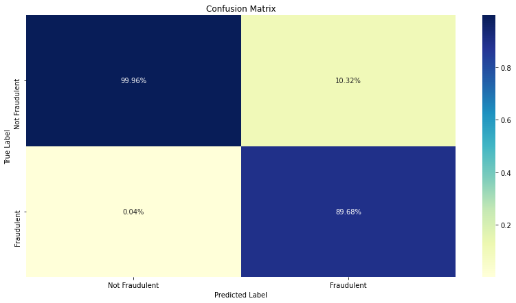
as expected the model does have some issue with classifiying fraudulent transactions, this can be addressed in multiple ways:
A deep dive into the intricacies of deploying custom models to Amazon SageMaker
How to create a new novel datasets from a few set of images.

Data Science Project

A Decentralized Application that simulates a bank using blockchain