Mastering Custom SageMaker Deployment: A Comprehensive Guide
A deep dive into the intricacies of deploying custom models to Amazon SageMaker

The goal of this project is to implement a bi-directional LSTM functional neural network that can classify named entities. the dataset has been extracted from GMB corpus and it is structured in a way that makes it easier to train a model for named entity recognition or part of speech tagging, however, we will be making use of only the named entity recognition part.
included entities:
# imports
import pandas as pd
import numpy as np
import matplotlib.pyplot as plt
from sklearn.model_selection import train_test_split
from keras.preprocessing.sequence import pad_sequences
from keras.utils import to_categorical
from keras.utils.vis_utils import plot_model
from numpy.random import seed
from itertools import chain
from tensorflow.keras import Model,Input
from tensorflow.keras.layers import LSTM,Embedding,Dense
from tensorflow.keras.layers import TimeDistributed, SpatialDropout1D,Bidirectional

plt.style.use('seaborn')
# getting the data
file = "../input/entity-annotated-corpus/ner_dataset.csv"
data = pd.read_csv(file, encoding = "latin1")

# drop the POS column because we dont need it
data = data.drop('POS', 1)
first lets take a look at our dataset by using the head function
data.head()
| Sentence # | Word | Tag | |
|---|---|---|---|
| 0 | Sentence: 1 | Thousands | O |
| 1 | NaN | of | O |
| 2 | NaN | demonstrators | O |
| 3 | NaN | have | O |
| 4 | NaN | marched | O |
the data has some na values, those values should be the number of the sentese, lets fix that
# Fill na
data = data.fillna(method = 'ffill')
seperate the words and tags into their own lists, later on this will be used for various actions including making the training and testing datasets and also when doing the prediction, another important number we need is the total number of tags which will be used for output sizes
words = list(set(data["Word"].values))
words.append("ENDPAD")
num_words = len(words)

print(f"Total number of unique words in dataset: {num_words}")
Total number of unique words in dataset: 35179
tags = list(set(data["Tag"].values))
num_tags = len(tags)
num_tags
print("List of tags: " + ', '.join([tag for tag in tags]))
print(f"Total Number of tags {num_tags}")
List of tags: B-nat, B-tim, I-org, B-art, B-org, I-eve, B-eve, B-per, I-per, I-geo, I-tim, B-gpe, I-gpe, I-nat, I-art, B-geo, O
Total Number of tags 17
lets make a class that will get get us a full sentense from our data, this is just for data exploration
class Get_sentence(object):
    def __init__(self,data):
        self.n_sent = 1
        self.data = data
        agg_func = lambda s:[(w, t) for w, t in zip(s["Word"].values.tolist(),
                                                    s["Tag"].values.tolist())]
        self.grouped = self.data.groupby("Sentence #").apply(agg_func)
        self.sentences = [s for s in self.grouped]
getter = Get_sentence(data)
sentence = getter.sentences
sentence[10]
[('In', 'O'),
 ('Beirut', 'B-geo'),
 (',', 'O'),
 ('a', 'O'),
 ('string', 'O'),
 ('of', 'O'),
 ('officials', 'O'),
 ('voiced', 'O'),
 ('their', 'O'),
 ('anger', 'O'),
 (',', 'O'),
 ('while', 'O'),
 ('at', 'O'),
 ('the', 'O'),
 ('United', 'B-org'),
 ('Nations', 'I-org'),
 ('summit', 'O'),
 ('in', 'O'),
 ('New', 'B-geo'),
 ('York', 'I-geo'),
 (',', 'O'),
 ('Prime', 'B-per'),
 ('Minister', 'O'),
 ('Fouad', 'B-per'),
 ('Siniora', 'I-per'),
 ('said', 'O'),
 ('the', 'O'),
 ('Lebanese', 'B-gpe'),
 ('people', 'O'),
 ('are', 'O'),
 ('resolute', 'O'),
 ('in', 'O'),
 ('preventing', 'O'),
 ('such', 'O'),
 ('attempts', 'O'),
 ('from', 'O'),
 ('destroying', 'O'),
 ('their', 'O'),
 ('spirit', 'O'),
 ('.', 'O')]
lets take a look at the distrbution of our words and tags in graphs which are easier to understand
plt.figure(figsize=(14,7))
plt.hist([len(s) for s in sentence],bins = 50)
plt.xlabel("Length of Sentences")
plt.show()

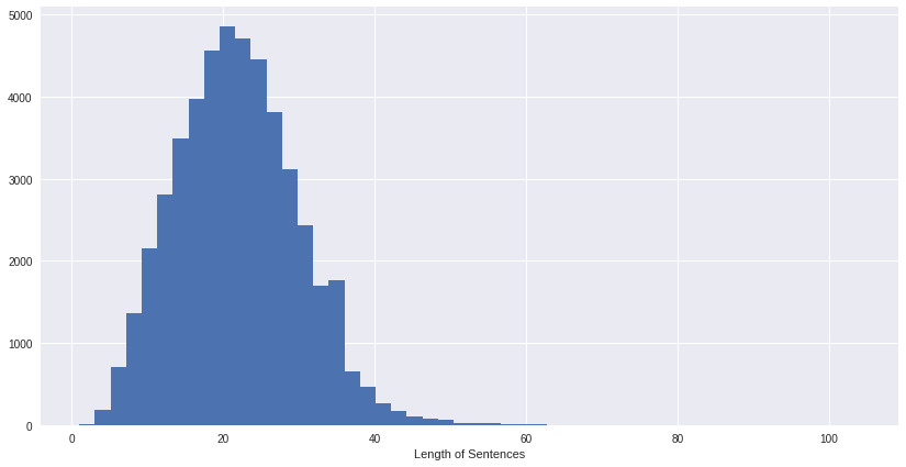
most of our sentenses have a length of 20 words, the longest sentense is around 63 words
plt.figure(figsize=(14, 7))
data.Tag[data.Tag != 'O']\
    .value_counts()\
    .plot\
    .barh();

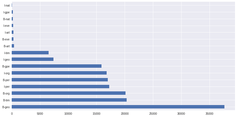
from the tags graph, we can observe that B-geo places are overrepresented, that might confuse the model, and also I-nat and I-gpe are almost non-existent in the dataset, we can already predict that the model might have issues classifying these 2 tags because of not enough training data for them.
When training a machine learning model we need to use sentences of an equal length, we are going to pad each of our sentences to a total length of 50 words, this might cut some sentences short but I believe thats fine since those are only a very few. an index mapping is a way we can link the tags and words numerically, each word has an index number and each tag has an index number as well, we can pass these number to our neural network and it will be able to learn with it efficiently, when we are doing prediction we use the predicted number as an index in our tags, words index list and get the actual tag, word.
word_idx = {w : i + 1 for i ,w in enumerate(words)}
tag_idx =  {t : i for i ,t in enumerate(tags)}
tag_idx
{'B-nat': 0,
 'B-tim': 1,
 'I-org': 2,
 'B-art': 3,
 'B-org': 4,
 'I-eve': 5,
 'B-eve': 6,
 'B-per': 7,
 'I-per': 8,
 'I-geo': 9,
 'I-tim': 10,
 'B-gpe': 11,
 'I-gpe': 12,
 'I-nat': 13,
 'I-art': 14,
 'B-geo': 15,
 'O': 16}
lets finally pad our sentenses using a max length of 50
max_len = 50
X = [[word_idx[w[0]] for w in s] for s in sentence]
X = pad_sequences(maxlen = max_len, sequences = X, padding = 'post', value = num_words - 1)

y = [[tag_idx[w[1]] for w in s] for s in sentence]
y = pad_sequences(maxlen = max_len, sequences = y, padding = 'post', value = tag_idx['O'])
y = [to_categorical(i, num_classes = num_tags) for i in  y]
now lets split the data into training and testing, we will use a testing dataset size of 10%, i belive that should be enough
x_train,x_test,y_train,y_test = train_test_split(X, y,test_size = 0.1, random_state = 1)
We will implement a functional model rather than a sequential one, the reason behind this is a functional model provided us with better accuracy in the current situation, we should always use the model that works best for the job, for example, a sequential Max Pooled LSTM did give me better results when doing a project about predicting COVID-19 cases, another reason is that a functional model is more flexible and allows us to have multiple inputs or output layers (thats more of a Keras API thing).
our loss measurement is categorical cross-entropy due to the prediction output and input being categorical labels in the end, for the optimizer, we will stick with adam because it works in most cases, we could adjust the learning rate for it but I don’t think that’s necessary.
input_word = Input(shape = (max_len,))
model = Embedding(input_dim = num_words, output_dim = max_len, input_length = max_len)(input_word)
model = SpatialDropout1D(0.1)(model)
model = Bidirectional(LSTM(units = 100,return_sequences = True, recurrent_dropout = 0.1))(model)
out = TimeDistributed(Dense(num_tags,activation = 'softmax'))(model)
model = Model(input_word,out)

model.compile(optimizer = 'adam',loss = 'categorical_crossentropy',metrics = ['accuracy'])
model.summary()
Model: "functional_1"
_________________________________________________________________
Layer (type)                 Output Shape              Param #
=================================================================
input_1 (InputLayer)         [(None, 50)]              0
_________________________________________________________________
embedding (Embedding)        (None, 50, 50)            1758950
_________________________________________________________________
spatial_dropout1d (SpatialDr (None, 50, 50)            0
_________________________________________________________________
bidirectional (Bidirectional (None, 50, 200)           120800
_________________________________________________________________
time_distributed (TimeDistri (None, 50, 17)            3417
=================================================================
Total params: 1,883,167
Trainable params: 1,883,167
Non-trainable params: 0
_________________________________________________________________
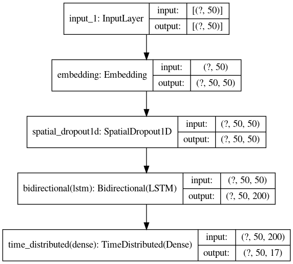
after building the model, the summary function shows us all the layers of the model and their parameters, inputs, and outputs, a better way to show such information is by using the plot_model method
we can see the final TimeDistributed layer outputs 50 tags of 17 types
plot_model(model, show_shapes = True)

Finally, we now train our model with these parameters
batch size: the number of words the model will train on at each time, the reason we chose 64 is sort of arbitrary, however, 64 * 540(total number of batches) = 34560 which is very close to our total number of words and tags, a higher batch number might speed up the training but will also reduce the accuracy.
epochs: the number of times the model will train through all the data, a higher number of epochs will not necessarily improve the accuracy. in fact, it might cause overfitting that is why we will stick to only 3 epochs.
validation split: the amount of data which will be used to validate the model during training, we will use 20% of our training dataset (do not confuse validation with testing, both are totally different things)
model.fit(x_train, np.array(y_train), batch_size = 64, verbose = 1, epochs = 3, validation_split = 0.2)
Epoch 1/3
540/540 [==============================] - 74s 138ms/step - loss: 0.2724 - accuracy: 0.9414 - val_loss: 0.1307 - val_accuracy: 0.9611
Epoch 2/3
540/540 [==============================] - 78s 145ms/step - loss: 0.0838 - accuracy: 0.9767 - val_loss: 0.0624 - val_accuracy: 0.9820
Epoch 3/3
540/540 [==============================] - 74s 136ms/step - loss: 0.0496 - accuracy: 0.9855 - val_loss: 0.0531 - val_accuracy: 0.9842
after the model has been trained the final loss is 0.439, and the final accuracy is 0.9845 which is 98.45% very high accuracy, I don’t think the model is overfitted because as we will see later on while predicting it has no problem working with foreign data.
Finally, let’s evaluate the model using our testing dataset
model.evaluate(x_test, np.array(y_test))
150/150 [==============================] - 3s 18ms/step - loss: 0.0554 - accuracy: 0.9840


[0.05543701350688934, 0.9840325117111206]
as you can see the testing dataset accuracy is very high as well, confirming that the model is not overfitted, now let’s try to tag random sentences from our training dataset and printing the original values compared to the values predicted by our model
rand_sent = np.random.randint(0, x_test.shape[0]) # get a random sentense
p = model.predict(np.array([x_test[rand_sent]]))
p = np.argmax(p, axis = -1)

y_true = np.argmax(np.array(y_test), axis = -1)[rand_sent] # get actual tags for random sentense

print("{:20}{:20}\t{}\n".format("Word", "True", "Pred"))
print("-" * 55)

for (w, t, pred) in zip(x_test[rand_sent], y_true, p[0]):
    print("{:20}{:20}\t{}".format(words[w - 1], tags[t], tags[pred]))
Word                True                	Pred

-------------------------------------------------------
The                 O                   	O
head                O                   	O
of                  O                   	O
the                 O                   	O
Public              B-org               	B-org
Agricultural        I-org               	I-org
Authority           I-org               	I-org
Sheikh              I-org               	I-org
Fahd                I-org               	I-org
Salem               I-org               	I-org
al-Sabah            I-org               	I-org
said                O                   	O
Thursday            B-tim               	B-tim
the                 O                   	O
cases               O                   	O
were                O                   	O
discovered          O                   	O
in                  O                   	O
two                 O                   	O
birds               O                   	O
and                 O                   	O
that                O                   	O
at                  O                   	O
least               O                   	O
one                 O                   	O
was                 O                   	O
a                   O                   	O
migrating           O                   	O
fowl                O                   	O
.                   O                   	O
lenient             O                   	O
lenient             O                   	O
lenient             O                   	O
lenient             O                   	O
lenient             O                   	O
lenient             O                   	O
lenient             O                   	O
lenient             O                   	O
lenient             O                   	O
lenient             O                   	O
lenient             O                   	O
lenient             O                   	O
lenient             O                   	O
lenient             O                   	O
lenient             O                   	O
lenient             O                   	O
lenient             O                   	O
lenient             O                   	O
lenient             O                   	O
lenient             O                   	O
now lets create a function so anyone can input their data and the model will do entity recognition on it!
def create_test_input_from_text(text):
    word_list = text.split(" ")
    x_new = []
    for word in word_list:
        x_new.append(word_idx[word])

    p = model.predict(np.array([x_new]))
    p = np.argmax(p, axis = -1)
    print("{:20}\t{}\n".format("Word", "Prediction"))
    print("-" * 35)

    for (w, pred) in zip(range(len(x_new)), p[0]):
        print("{:20}\t{}".format(word_list[w], tags[pred]))
test_inputs = "the weather in London is very hot"
create_test_input_from_text(test_inputs)
Word                	Prediction

------------------------------
the                 	O
weather             	O
in                  	O
London              	B-geo
is                  	O
very                	O
hot                 	O
test_inputs = "my friend Mohammed is travelling to Oman"
create_test_input_from_text(test_inputs)
Word                	Prediction

------------------------------
my                  	O
friend              	O
Mohammed            	B-per
is                  	O
travelling          	B-geo
to                  	O
Oman                	I-geo

A deep dive into the intricacies of deploying custom models to Amazon SageMaker

How to create a new novel datasets from a few set of images.

Data Science Project

Data Science Project