
Mastering Custom SageMaker Deployment: A Comprehensive Guide
A deep dive into the intricacies of deploying custom models to Amazon SageMaker

the dataset is saved as a csv containing pixel values for 784 pixels resulting in images of size 28 _ 28 _ 1 with one color channel.
!pip -q install torchsummary
# imports
import string
import pandas as pd
import numpy as np
import seaborn as sns
import matplotlib
import matplotlib.pyplot as plt
import torch
import torch.nn as nn
import torch.nn.functional as F
import torchvision.transforms as T
from torch.utils.data import DataLoader, Dataset
from torchvision.utils import make_grid
from sklearn.metrics import accuracy_score, confusion_matrix, classification_report
from sklearn.model_selection import train_test_split
from torchsummary import summary
from tqdm import tqdm

# some settings
# set background color to white
matplotlib.rcParams['figure.facecolor'] = '#ffffff'

# set default figure size
matplotlib.rcParams['figure.figsize'] = (15, 7)
# read data
train_df = pd.read_csv("../input/sign-language-mnist/sign_mnist_train/sign_mnist_train.csv")
test_df = pd.read_csv("../input/sign-language-mnist/sign_mnist_test/sign_mnist_test.csv")
each row in the data represents an image with the first column being the label for the image
# checkout data
train_df.head()
| label | pixel1 | pixel2 | pixel3 | pixel4 | pixel5 | pixel6 | pixel7 | pixel8 | pixel9 | ... | pixel775 | pixel776 | pixel777 | pixel778 | pixel779 | pixel780 | pixel781 | pixel782 | pixel783 | pixel784 | |
|---|---|---|---|---|---|---|---|---|---|---|---|---|---|---|---|---|---|---|---|---|---|
| 0 | 3 | 107 | 118 | 127 | 134 | 139 | 143 | 146 | 150 | 153 | ... | 207 | 207 | 207 | 207 | 206 | 206 | 206 | 204 | 203 | 202 |
| 1 | 6 | 155 | 157 | 156 | 156 | 156 | 157 | 156 | 158 | 158 | ... | 69 | 149 | 128 | 87 | 94 | 163 | 175 | 103 | 135 | 149 |
| 2 | 2 | 187 | 188 | 188 | 187 | 187 | 186 | 187 | 188 | 187 | ... | 202 | 201 | 200 | 199 | 198 | 199 | 198 | 195 | 194 | 195 |
| 3 | 2 | 211 | 211 | 212 | 212 | 211 | 210 | 211 | 210 | 210 | ... | 235 | 234 | 233 | 231 | 230 | 226 | 225 | 222 | 229 | 163 |
| 4 | 13 | 164 | 167 | 170 | 172 | 176 | 179 | 180 | 184 | 185 | ... | 92 | 105 | 105 | 108 | 133 | 163 | 157 | 163 | 164 | 179 |
5 rows × 785 columns
train_df.describe()
| label | pixel1 | pixel2 | pixel3 | pixel4 | pixel5 | pixel6 | pixel7 | pixel8 | pixel9 | ... | pixel775 | pixel776 | pixel777 | pixel778 | pixel779 | pixel780 | pixel781 | pixel782 | pixel783 | pixel784 | |
|---|---|---|---|---|---|---|---|---|---|---|---|---|---|---|---|---|---|---|---|---|---|
| count | 27455.000000 | 27455.000000 | 27455.000000 | 27455.000000 | 27455.000000 | 27455.000000 | 27455.000000 | 27455.000000 | 27455.000000 | 27455.000000 | ... | 27455.000000 | 27455.000000 | 27455.000000 | 27455.000000 | 27455.000000 | 27455.000000 | 27455.000000 | 27455.000000 | 27455.000000 | 27455.000000 |
| mean | 12.318813 | 145.419377 | 148.500273 | 151.247714 | 153.546531 | 156.210891 | 158.411255 | 160.472154 | 162.339683 | 163.954799 | ... | 141.104863 | 147.495611 | 153.325806 | 159.125332 | 161.969259 | 162.736696 | 162.906137 | 161.966454 | 161.137898 | 159.824731 |
| std | 7.287552 | 41.358555 | 39.942152 | 39.056286 | 38.595247 | 37.111165 | 36.125579 | 35.016392 | 33.661998 | 32.651607 | ... | 63.751194 | 65.512894 | 64.427412 | 63.708507 | 63.738316 | 63.444008 | 63.509210 | 63.298721 | 63.610415 | 64.396846 |
| min | 0.000000 | 0.000000 | 0.000000 | 0.000000 | 0.000000 | 0.000000 | 0.000000 | 0.000000 | 0.000000 | 0.000000 | ... | 0.000000 | 0.000000 | 0.000000 | 0.000000 | 0.000000 | 0.000000 | 0.000000 | 0.000000 | 0.000000 | 0.000000 |
| 25% | 6.000000 | 121.000000 | 126.000000 | 130.000000 | 133.000000 | 137.000000 | 140.000000 | 142.000000 | 144.000000 | 146.000000 | ... | 92.000000 | 96.000000 | 103.000000 | 112.000000 | 120.000000 | 125.000000 | 128.000000 | 128.000000 | 128.000000 | 125.500000 |
| 50% | 13.000000 | 150.000000 | 153.000000 | 156.000000 | 158.000000 | 160.000000 | 162.000000 | 164.000000 | 165.000000 | 166.000000 | ... | 144.000000 | 162.000000 | 172.000000 | 180.000000 | 183.000000 | 184.000000 | 184.000000 | 182.000000 | 182.000000 | 182.000000 |
| 75% | 19.000000 | 174.000000 | 176.000000 | 178.000000 | 179.000000 | 181.000000 | 182.000000 | 183.000000 | 184.000000 | 185.000000 | ... | 196.000000 | 202.000000 | 205.000000 | 207.000000 | 208.000000 | 207.000000 | 207.000000 | 206.000000 | 204.000000 | 204.000000 |
| max | 24.000000 | 255.000000 | 255.000000 | 255.000000 | 255.000000 | 255.000000 | 255.000000 | 255.000000 | 255.000000 | 255.000000 | ... | 255.000000 | 255.000000 | 255.000000 | 255.000000 | 255.000000 | 255.000000 | 255.000000 | 255.000000 | 255.000000 | 255.000000 |
8 rows × 785 columns
train_df.info()
<class 'pandas.core.frame.DataFrame'>
RangeIndex: 27455 entries, 0 to 27454
Columns: 785 entries, label to pixel784
dtypes: int64(785)
memory usage: 164.4 MB
test_df.info()
<class 'pandas.core.frame.DataFrame'>
RangeIndex: 7172 entries, 0 to 7171
Columns: 785 entries, label to pixel784
dtypes: int64(785)
memory usage: 43.0 MB
# create a dictionary for mapping numbers to letters
alpha_dict = {idx:letter for idx, letter in enumerate(string.ascii_lowercase)}
alpha_dict
{0: 'a',
 1: 'b',
 2: 'c',
 3: 'd',
 4: 'e',
 5: 'f',
 6: 'g',
 7: 'h',
 8: 'i',
 9: 'j',
 10: 'k',
 11: 'l',
 12: 'm',
 13: 'n',
 14: 'o',
 15: 'p',
 16: 'q',
 17: 'r',
 18: 's',
 19: 't',
 20: 'u',
 21: 'v',
 22: 'w',
 23: 'x',
 24: 'y',
 25: 'z'}
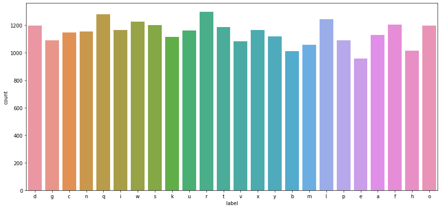
# check class distribution
# convert to actual letters using dict
alpha_labels = train_df.label.apply(lambda x: alpha_dict[x])
sns.countplot(x=alpha_labels)
plt.show()
# create custom pytorch dataset class
class SignDataset(Dataset) :
    def __init__(self, img, label) :
        self.classes = np.array(label)
        img = img / 255.0
        self.img = np.array(img).reshape(-1, 28, 28, 1)

        self.transform = T.Compose([
            T.ToTensor()
        ])

    def __len__(self) :
        return len(self.img)

    def __getitem__(self, index) :
        label = self.classes[index]
        img = self.img[index]
        img = self.transform(img)

        label = torch.LongTensor([label])
        img = img.float()

        return img, label
# create datasets
train_set = SignDataset(train_df.drop('label', axis=1), train_df['label'])
test_set = SignDataset(test_df.drop('label', axis=1), test_df['label'])
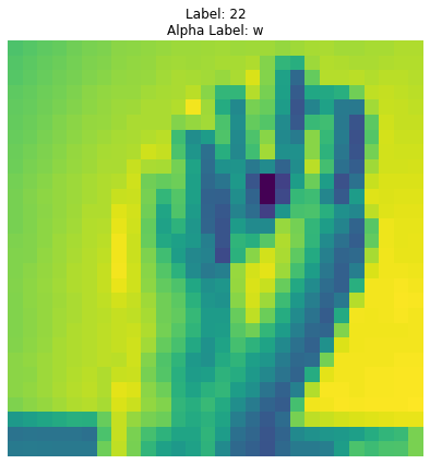
# show a single image
def show_image(img, label, dataset):
    plt.imshow(img.permute(1, 2, 0))
    plt.axis('off')
    plt.title(f"Label: {dataset.classes[label]}\nAlpha Label: {alpha_dict[dataset.classes[label]]}")
show_image(*train_set[4], train_set)
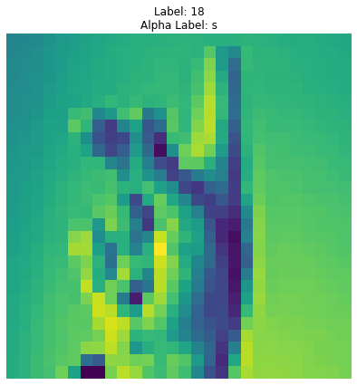
show_image(*train_set[45], train_set)
batch_size = 128
train_dl = DataLoader(train_set, batch_size=batch_size)
test_dl = DataLoader(test_set, batch_size=batch_size)
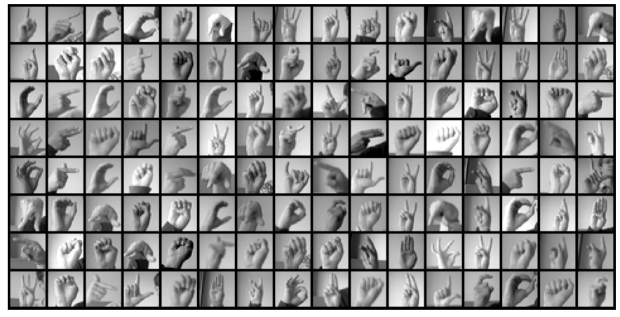
# visualize a batch of images
def show_batch(dl):
    for images, labels in dl:
        fig, ax = plt.subplots(figsize=(20, 8))
        ax.set_xticks([]); ax.set_yticks([])
        ax.imshow(make_grid(images, nrow=16).permute(1, 2, 0))
        break
# show a batch of images (128 images)
show_batch(train_dl)
# convlutional block with batchnorm, max pooling and dropout
def conv_block(in_channels, out_channels, pool=False, drop=False):
    layers = [nn.Conv2d(in_channels, out_channels, kernel_size=3, padding=1),
              nn.BatchNorm2d(out_channels),
              nn.ReLU(inplace=True)]
    if pool: layers.append(nn.MaxPool2d(2))
    if drop: layers.append(nn.Dropout())
    return nn.Sequential(*layers)
# network architecture
class SignConvNet(nn.Module):
    def __init__(self, in_channels, out_classes):
        super().__init__()
        self.conv1 = conv_block(in_channels, 16)
        self.conv2 = conv_block(16, 32, pool=True)
        self.conv3 = conv_block(32, 64, pool=True, drop=True)
        self.fc =  nn.Sequential(*[
                        nn.Flatten(),
                        nn.Linear(7 * 7 * 64, out_classes)
                    ])

    def forward(self, img):
        img = self.conv1(img)
        img = self.conv2(img)
        img = self.conv3(img)
        return self.fc(img)
# get number of classes
num_classes = len(alpha_dict)

# set device
device = torch.device('cuda' if torch.cuda.is_available() else 'cpu')

# create model, optim  and loss
model = SignConvNet(1, num_classes).to(device)
criterion = nn.CrossEntropyLoss().to(device)
optim = torch.optim.Adam(model.parameters(), lr=1e-3)

# checkout model layer output shapes, and memory usage
summary(model, (1, 28, 28))
----------------------------------------------------------------
        Layer (type)               Output Shape         Param #
================================================================
            Conv2d-1           [-1, 16, 28, 28]             160
       BatchNorm2d-2           [-1, 16, 28, 28]              32
              ReLU-3           [-1, 16, 28, 28]               0
            Conv2d-4           [-1, 32, 28, 28]           4,640
       BatchNorm2d-5           [-1, 32, 28, 28]              64
              ReLU-6           [-1, 32, 28, 28]               0
         MaxPool2d-7           [-1, 32, 14, 14]               0
            Conv2d-8           [-1, 64, 14, 14]          18,496
       BatchNorm2d-9           [-1, 64, 14, 14]             128
             ReLU-10           [-1, 64, 14, 14]               0
        MaxPool2d-11             [-1, 64, 7, 7]               0
          Dropout-12             [-1, 64, 7, 7]               0
          Flatten-13                 [-1, 3136]               0
           Linear-14                   [-1, 26]          81,562
================================================================
Total params: 105,082
Trainable params: 105,082
Non-trainable params: 0
----------------------------------------------------------------
Input size (MB): 0.00
Forward/backward pass size (MB): 1.27
Params size (MB): 0.40
Estimated Total Size (MB): 1.67
----------------------------------------------------------------
epochs = 10
losses = []
for epoch in range(epochs):
    # for custom progress bar
    with tqdm(train_dl, unit="batch") as tepoch:
        epoch_loss = 0
        epoch_acc = 0
        for data, target in tepoch:
            tepoch.set_description(f"Epoch {epoch + 1}")
            data, target = data.to(device), target.to(device) # move input to GPU
            out = model(data)
            loss = criterion(out, target.squeeze())
            epoch_loss += loss.item()
            loss.backward()
            optim.step()
            optim.zero_grad()
            tepoch.set_postfix(loss = loss.item()) # show loss and per batch of data
    losses.append(epoch_loss)
Epoch 1: 100%|██████████| 215/215 [00:02<00:00, 81.52batch/s, loss=0.00943]
Epoch 2: 100%|██████████| 215/215 [00:02<00:00, 81.32batch/s, loss=0.00608]
Epoch 3: 100%|██████████| 215/215 [00:03<00:00, 62.13batch/s, loss=0.00424]
Epoch 4: 100%|██████████| 215/215 [00:02<00:00, 80.00batch/s, loss=0.0211]
Epoch 5: 100%|██████████| 215/215 [00:02<00:00, 81.77batch/s, loss=0.00428]
Epoch 6: 100%|██████████| 215/215 [00:02<00:00, 81.05batch/s, loss=0.00279]
Epoch 7: 100%|██████████| 215/215 [00:02<00:00, 75.95batch/s, loss=0.0431]
Epoch 8: 100%|██████████| 215/215 [00:02<00:00, 80.23batch/s, loss=0.00375]
Epoch 9: 100%|██████████| 215/215 [00:02<00:00, 80.76batch/s, loss=0.000472]
Epoch 10: 100%|██████████| 215/215 [00:02<00:00, 80.97batch/s, loss=0.00668]
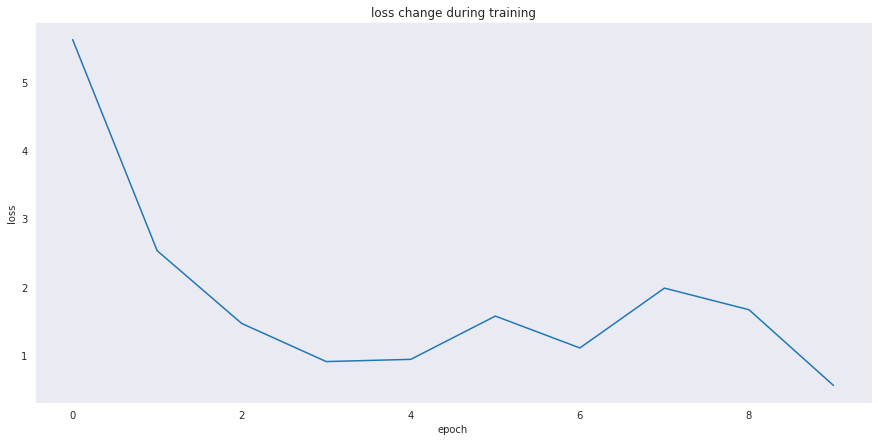
# plot losses
sns.set_style("dark")
sns.lineplot(data=losses).set(title="loss change during training", xlabel="epoch", ylabel="loss")
plt.show()
# predict on testing data samples (the accuracy here is batch accuracy)
y_pred_list = []
y_true_list = []
with torch.no_grad():
    with tqdm(test_dl, unit="batch") as tepoch:
        for inp, labels in tepoch:
            inp, labels = inp.to(device), labels.to(device)
            y_test_pred = model(inp)
            _, y_pred_tag = torch.max(y_test_pred, dim = 1)
            y_pred_list.append(y_pred_tag.cpu().numpy())
            y_true_list.append(labels.cpu().numpy())
100%|██████████| 57/57 [00:00<00:00, 180.71batch/s]
# flatten prediction and true lists
flat_pred = []
flat_true = []
for i in range(len(y_pred_list)):
    for j in range(len(y_pred_list[i])):
        flat_pred.append(y_pred_list[i][j])
        flat_true.append(y_true_list[i][j])

print(f"number of testing samples results: {len(flat_pred)}")
number of testing samples results: 7172
# calculate total testing accuracy
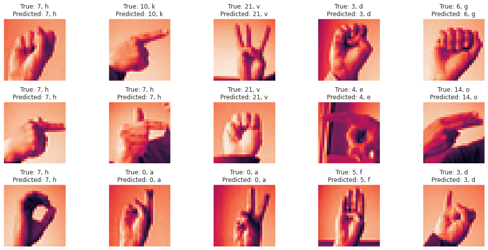
print(f"Testing accuracy is: {accuracy_score(flat_true, flat_pred) * 100:.2f}%")
Testing accuracy is: 94.19%
# Display 15 random picture of the dataset with their labels
inds = np.random.randint(len(test_set), size=15)
fig, axes = plt.subplots(nrows=3, ncols=5, figsize=(15, 7),
                        subplot_kw={'xticks': [], 'yticks': []})

for i, ax in zip(inds, axes.flat):
    img, label = test_set[i]
    ax.imshow(img.permute(1, 2, 0))
    dict_real = alpha_dict[test_set.classes[label]]
    dict_pred = alpha_dict[test_set.classes[flat_pred[i]]]
    ax.set_title(f"True: {test_set.classes[label]}, {dict_real}\nPredicted: {test_set.classes[flat_pred[i]]}, {dict_pred}")
plt.tight_layout()
plt.show()
# classification report
print(classification_report(flat_true, flat_pred))
              precision    recall  f1-score   support

           0       1.00      1.00      1.00       331
           1       1.00      0.92      0.96       432
           2       1.00      0.98      0.99       310
           3       0.94      0.97      0.95       245
           4       0.97      0.99      0.98       498
           5       0.88      1.00      0.93       247
           6       0.90      0.94      0.92       348
           7       0.91      0.93      0.92       436
           8       0.97      0.95      0.96       288
          10       0.94      0.93      0.94       331
          11       0.99      1.00      1.00       209
          12       0.91      0.94      0.92       394
          13       0.88      0.81      0.84       291
          14       1.00      0.98      0.99       246
          15       0.95      1.00      0.98       347
          16       0.97      0.99      0.98       164
          17       0.82      0.86      0.84       144
          18       0.97      0.93      0.95       246
          19       0.87      0.80      0.84       248
          20       0.99      0.89      0.94       266
          21       0.94      0.91      0.93       346
          22       0.83      0.96      0.89       206
          23       0.90      0.96      0.93       267
          24       0.97      0.92      0.95       332

    accuracy                           0.94      7172
   macro avg       0.94      0.94      0.94      7172
weighted avg       0.94      0.94      0.94      7172
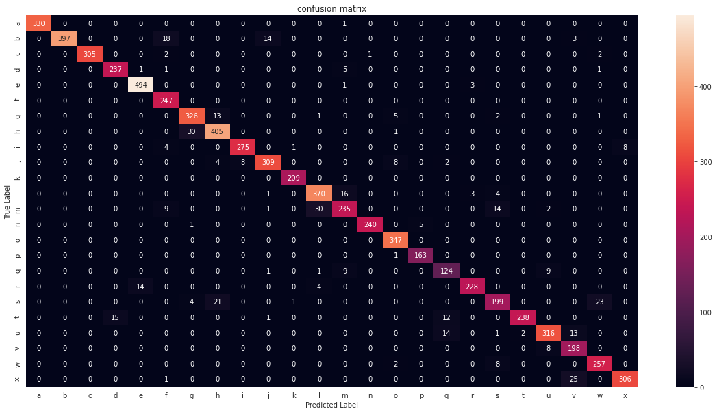
# plot confusion matrix
confusion_matrix_df = pd.DataFrame(confusion_matrix(flat_true, flat_pred)).rename(columns=alpha_dict, index=alpha_dict)
plt.figure(figsize=(20, 10))
sns.heatmap(confusion_matrix_df, annot=True, fmt='').set(title="confusion matrix", xlabel="Predicted Label", ylabel="True Label")
plt.show()
A deep dive into the intricacies of deploying custom models to Amazon SageMaker
How to create a new novel datasets from a few set of images.
Data Science Project

Data Science Project